Solución
Apartado a
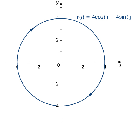
Esta función describe una circunferencia.
Para encontrar el vector normal principal unitario, primero debemos encontrarel vector tangente unitario T ( t ) \bold{T}(t) T ( t )
T ( t ) = r ′ ( t ) ∥ r ′ ( t ) ∥ = − 4 s e n t i − 4 c o s t j ( − 4 s e n t ) 2 + ( − 4 c o s t ) 2 = − 4 s e n t i − 4 c o s t j 16 s e n 2 t + 16 c o s 2 t = − 4 s e n t i − 4 c o s t j 16 ( s e n 2 t + c o s 2 t ) = − 4 s e n t i − 4 c o s t j 4 = − s e n t i − c o s t j \begin{aligned}
\bold{T}(t) &= \frac{\bold{r'}(t)}{\|\bold{r'}(t)\|}\\
&= \frac{-4sent\bold{i}-4cost\bold{j}}{\sqrt{(-4sent)^2+(-4cost)^2}}\\
&= \frac{-4sent\bold{i}-4cost\bold{j}}{\sqrt{16sen^2t+16cos^2t}}\\
&= \frac{-4sent\bold{i}-4cost\bold{j}}{\sqrt{16(sen^2t+cos^2t)}}\\
&= \frac{-4sent\bold{i}-4cost\bold{j}}{4}\\
&= -sent\bold{i}-cost\bold{j}
\end{aligned} T ( t ) = ∥ r ′ ( t ) ∥ r ′ ( t ) = ( − 4 se n t ) 2 + ( − 4 cos t ) 2 − 4 se n t i − 4 cos t j = 16 se n 2 t + 16 co s 2 t − 4 se n t i − 4 cos t j = 16 ( se n 2 t + co s 2 t ) − 4 se n t i − 4 cos t j = 4 − 4 se n t i − 4 cos t j = − se n t i − cos t j A continuación, usamos la ecuación 3.18:
N ( t ) = T ′ ( t ) ∥ T ′ ( t ) ∥ = − c o s t i + s e n t j ( − c o s t ) 2 + ( s e n t ) 2 = − c o s t i + s e n t j s e n 2 t + c o s 2 t = − c o s t i + s e n t j \begin{aligned}
\bold{N}(t) &= \frac{\bold{T'}(t)}{\|\bold{T'}(t)\|}\\
&= \frac{-cost\bold{i}+sent\bold{j}}{\sqrt{(-cost)^2+(sent)^2}}\\
&= \frac{-cost\bold{i}+sent\bold{j}}{\sqrt{sen^2t+cos^2t}}\\
&= -cost\bold{i}+sent\bold{j}
\end{aligned} N ( t ) = ∥ T ′ ( t ) ∥ T ′ ( t ) = ( − cos t ) 2 + ( se n t ) 2 − cos t i + se n t j = se n 2 t + co s 2 t − cos t i + se n t j = − cos t i + se n t j Observa que el vector tangente unitario y el vector normal principal unitario son ortogonales entre sí para todos los valores de t t t
T ( t ) ⋅ N ( t ) = ⟨ − s e n t , − c o s t ⟩ ⋅ ⟨ − c o s t , s e n t ⟩ = s e n t c o s t − c o s t s e n t = 0 \begin{aligned}
\bold{T}(t)\cdot\bold{N}(t) &= \lang −sent,−cost\rang\cdot\lang −cost,sent\rang\\
&= sentcost−costsent\\
&= 0
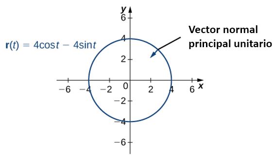
\end{aligned} T ( t ) ⋅ N ( t ) = ⟨ − se n t , − cos t ⟩ ⋅ ⟨ − cos t , se n t ⟩ = se n t cos t − cos t se n t = 0 Además, el vector normal principal unitario apunta hacia el centro del círculo desde cada punto del círculo. Dado que r ( t ) \bold{r}(t) r ( t )
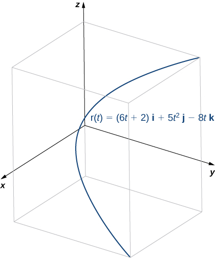
Apartado b
Esta función se ve así:
Para encontrar el vector normal principal unitario, primero debemos encontrarel vector tangente unitario T ( t ) \bold{T}(t) T ( t )
T ( t ) = r ′ ( t ) ∥ r ′ ( t ) ∥ = 6 i + 10 t j − 8 k 6 2 + ( 10 t ) 2 + ( − 8 ) 2 = 6 i + 10 t j − 8 k 36 + 100 t 2 + 64 = 6 i + 10 t j − 8 k 100 ( t 2 + 1 ) = 3 i + 5 t j − 4 k 5 t 2 + 1 = 3 5 ( t 2 + 1 ) − 1 / 2 i − t ( t 2 + 1 ) − 1 / 2 j − 4 5 ( t 2 + 1 ) − 1 / 2 k \begin{aligned}
\bold{T}(t) &= \frac{\bold{r'}(t)}{\|\bold{r'}(t)\|}\\
&= \frac{6\bold{i}+10t\bold{j}−8\bold{k}}{\sqrt{6^2+(10t)^2+(-8)^2}}\\
&= \frac{6\bold{i}+10t\bold{j}−8\bold{k}}{\sqrt{36+100t^2+64}}\\
&= \frac{6\bold{i}+10t\bold{j}−8\bold{k}}{\sqrt{100(t^2+1)}}\\
&= \frac{3\bold{i}+5t\bold{j}−4\bold{k}}{5\sqrt{t^2+1}}\\
&= \frac{3}{5}(t^2+1)^{-1/2}\bold{i} - t(t^2+1)^{-1/2}\bold{j} - \frac{4}{5}(t^2+1)^{-1/2}\bold{k}
\end{aligned} T ( t ) = ∥ r ′ ( t ) ∥ r ′ ( t ) = 6 2 + ( 10 t ) 2 + ( − 8 ) 2 6 i + 10 t j − 8 k = 36 + 100 t 2 + 64 6 i + 10 t j − 8 k = 100 ( t 2 + 1 ) 6 i + 10 t j − 8 k = 5 t 2 + 1 3 i + 5 t j − 4 k = 5 3 ( t 2 + 1 ) − 1/2 i − t ( t 2 + 1 ) − 1/2 j − 5 4 ( t 2 + 1 ) − 1/2 k A continuación, calculamos T ′ ( t ) \bold{T}'(t) T ′ ( t ) ∥ T ′ ( t ) ∥ \|\bold{T}'(t)\| ∥ T ′ ( t ) ∥
T ′ ( t ) = 3 5 ( − 1 2 ) ( t 2 + 1 ) − 3 / 2 ( 2 t ) i + ( ( t 2 + 1 ) − 1 / 2 − t ( 1 2 ) ( t 2 + 1 ) − 3 / 2 ( 2 t ) j − 4 5 ( − 1 2 ) ( t 2 + 1 ) − 3 / 2 ( 2 t ) k = − 3 t 5 ( t 2 + 1 ) 3 / 2 i − 1 ( t 2 + 1 ) 3 / 2 j + 4 t 5 ( t 2 + 1 ) 3 / 2 k ∥ T ′ ( t ) ∥ = ( − 3 t 5 ( t 2 + 1 ) 3 / 2 ) 2 + ( − 1 ( t 2 + 1 ) 3 / 2 ) 2 + ( 4 t 5 ( t 2 + 1 ) 3 / 2 ) 2 = 9 t 2 25 ( t 2 + 1 ) 3 + 1 ( t 2 + 1 ) 3 + 16 t 2 25 ( t 2 + 1 ) 3 = 25 t 2 + 25 25 ( t 2 + 1 ) 3 = 1 ( t 2 + 1 ) 2 = 1 t 2 + 1 \begin{aligned}
\bold{T}'(t) &= \frac{3}{5}\big(-\frac{1}{2}\big)(t^2+1)^{-3/2}(2t)\bold{i}
&+\bigg((t^2+1)^{-1/2} -t\big(\frac{1}{2}\big)(t^2+1)^{-3/2}(2t)\bold{j}\\
& -\frac{4}{5}\big(-\frac{1}{2}\big)(t^2+1)^{-3/2}(2t)\bold{k}\\
&= -\frac{3t}{5(t^2+1)^{3/2}}\bold{i} - \frac{1}{(t^2+1)^{3/2}}\bold{j} + \frac{4t}{5(t^2+1)^{3/2}}\bold{k}\\
\|\bold{T′}(t)\| &= \sqrt{\Bigg(-\frac{3t}{5(t^2+1)^{3/2}} \Bigg)^2 + \Bigg(- \frac{1}{(t^2+1)^{3/2}} \Bigg)^2 + \Bigg(\frac{4t}{5(t^2+1)^{3/2}} \Bigg)^2}\\
&= \sqrt{\frac{9t^2}{25(t^2+1)^3} + \frac{1}{(t^2+1)^3} + \frac{16t^2}{25(t^2+1)^3}}\\
&= \sqrt{\frac{25t^2+25}{25(t^2+1)^3}}\\
&= \sqrt{\frac{1}{(t^2+1)^2}}\\
&= \frac{1}{t^2+1}
\end{aligned} T ′ ( t ) ∥ T′ ( t ) ∥ = 5 3 ( − 2 1 ) ( t 2 + 1 ) − 3/2 ( 2 t ) i − 5 4 ( − 2 1 ) ( t 2 + 1 ) − 3/2 ( 2 t ) k = − 5 ( t 2 + 1 ) 3/2 3 t i − ( t 2 + 1 ) 3/2 1 j + 5 ( t 2 + 1 ) 3/2 4 t k = ( − 5 ( t 2 + 1 ) 3/2 3 t ) 2 + ( − ( t 2 + 1 ) 3/2 1 ) 2 + ( 5 ( t 2 + 1 ) 3/2 4 t ) 2 = 25 ( t 2 + 1 ) 3 9 t 2 + ( t 2 + 1 ) 3 1 + 25 ( t 2 + 1 ) 3 16 t 2 = 25 ( t 2 + 1 ) 3 25 t 2 + 25 = ( t 2 + 1 ) 2 1 = t 2 + 1 1 + ( ( t 2 + 1 ) − 1/2 − t ( 2 1 ) ( t 2 + 1 ) − 3/2 ( 2 t ) j Por lo tanto, de acuerdo con la Ecuación 3.18:
N ( t ) = T ′ ( t ) ∥ T ′ ( t ) ∥ = ( − 3 t 5 ( t 2 + 1 ) 3 / 2 i − 1 ( t 2 + 1 ) 3 / 2 j + 4 t 5 ( t 2 + 1 ) 3 / 2 k ) ( t 2 + 1 ) = − 3 t 5 ( t 2 + 1 ) 1 / 2 i − 5 5 ( t 2 + 1 ) 1 / 2 j + 4 t 5 ( t 2 + 1 ) 1 / 2 k = − 3 t i + 5 j − 4 t k 5 t 2 + 1 \begin{aligned}
\bold{N}(t) &= \frac{\bold{T'}(t)}{\|\bold{T'}(t)\|}\\
&= \Bigg(-\frac{3t}{5(t^2+1)^{3/2}}\bold{i} - \frac{1}{(t^2+1)^{3/2}}\bold{j} + \frac{4t}{5(t^2+1)^{3/2}}\bold{k}\Bigg)(t^2+1)\\
&= -\frac{3t}{5(t^2+1)^{1/2}}\bold{i} - \frac{5}{5(t^2+1)^{1/2}}\bold{j} +\frac{4t}{5(t^2+1)^{1/2}}\bold{k}\\
&= -\frac{3t\bold{i}+5\bold{j}−4t\bold{k}}{5\sqrt{t^2+1}}
\end{aligned} N ( t ) = ∥ T ′ ( t ) ∥ T ′ ( t ) = ( − 5 ( t 2 + 1 ) 3/2 3 t i − ( t 2 + 1 ) 3/2 1 j + 5 ( t 2 + 1 ) 3/2 4 t k ) ( t 2 + 1 ) = − 5 ( t 2 + 1 ) 1/2 3 t i − 5 ( t 2 + 1 ) 1/2 5 j + 5 ( t 2 + 1 ) 1/2 4 t k = − 5 t 2 + 1 3 t i + 5 j − 4 t k Una vez más, el vector tangente unitario y el vector normal principal unitario son ortogonales entre sí para todos los valores de t t t
T ( t ) ⋅ N ( t ) = ( 3 i − 5 t j − 4 k 5 t 2 + 1 ) ⋅ ( − 3 t i + 5 j − 4 t k 5 t 2 + 1 ) = 3 ( − 3 t ) − 5 t ( − 5 ) − 4 ( 4 t ) 25 ( t 2 + 1 ) = − 9 t + 25 t − 16 t 25 ( t 2 + 1 ) = 0 \begin{aligned}
\bold{T}(t)\cdot\bold{N}(t) &= \bigg(\frac{3\bold{i}−5t\bold{j}−4\bold{k}}{5\sqrt{t^2+1}}\bigg)\cdot\bigg(-\frac{3t\bold{i}+5\bold{j}−4t\bold{k}}{5\sqrt{t^2+1}}\bigg)\\
&= \frac{3(−3t)−5t(−5)−4(4t)}{25\big(t^2+1\big)}\\
&= \frac{−9t+25t−16t}{25\big(t^2+1\big)}\\
&= 0
\end{aligned} T ( t ) ⋅ N ( t ) = ( 5 t 2 + 1 3 i − 5 t j − 4 k ) ⋅ ( − 5 t 2 + 1 3 t i + 5 j − 4 t k ) = 25 ( t 2 + 1 ) 3 ( − 3 t ) − 5 t ( − 5 ) − 4 ( 4 t ) = 25 ( t 2 + 1 ) − 9 t + 25 t − 16 t = 0 Por último, dado que r ( t ) \bold{r}(t) r ( t )
B ( t ) = T ( t ) × N ( t ) = ∣ i j k 3 5 t 2 + 1 − 5 t 5 t 2 + 1 − 4 5 t 2 + 1 − 3 t 5 t 2 + 1 − 5 5 t 2 + 1 4 t 5 t 2 + 1 ∣ = ( ( − 5 t 5 t 2 + 1 ) ( 4 t 5 t 2 + 1 ) − ( − 4 5 t 2 + 1 ) ( − 5 5 t 2 + 1 ) ) i − ( ( 3 5 t 2 + 1 ) ( 4 t 5 t 2 + 1 ) − ( − 4 5 t 2 + 1 ) ( − 3 t 5 t 2 + 1 ) ) j + ( ( 3 5 t 2 + 1 ) ( − 5 5 t 2 + 1 ) − ( − 5 t 5 t 2 + 1 ) ( − 3 t 5 t 2 + 1 ) ) k = ( − 20 t 2 − 20 25 ( t 2 + 1 ) ) i + ( − 15 − 15 t 2 25 ( t 2 + 1 ) ) k = − 20 ( t 2 + 1 25 ( t 2 + 1 ) ) i − 15 ( t 2 + 1 25 ( t 2 + 1 ) ) k = − 4 5 i − 3 5 k \begin{aligned}
\bold{B}(t) &= \bold{T}(t)\times\bold{N}(t)\\
&= \begin{vmatrix} \bold{i} & \bold{j} & \bold{k}\\ \\
\frac{3}{5\sqrt{t^2+1}} & -\frac{5t}{5\sqrt{t^2+1}} & -\frac{4}{5\sqrt{t^2+1}}\\ \\
-\frac{3t}{5\sqrt{t^2+1}} & -\frac{5}{5\sqrt{t^2+1}} & \frac{4t}{5\sqrt{t^2+1}}
\end{vmatrix}\\
&= \Bigg(\bigg(-\frac{5t}{5\sqrt{t^2+1}}\bigg)\bigg(\frac{4t}{5\sqrt{t^2+1}}\bigg) - \bigg(-\frac{4}{5\sqrt{t^2+1}}\bigg)\bigg(-\frac{5}{5\sqrt{t^2+1}}\bigg)\Bigg)\bold{i}\\
& \;\;\;\;-\Bigg(\bigg(\frac{3}{5\sqrt{t^2+1}}\bigg)\bigg(\frac{4t}{5\sqrt{t^2+1}}\bigg) - \bigg(-\frac{4}{5\sqrt{t^2+1}}\bigg)\bigg(-\frac{3t}{5\sqrt{t^2+1}}\bigg)\Bigg)\bold{j}\\
& \;\;\;\; +\Bigg(\bigg(\frac{3}{5\sqrt{t^2+1}}\bigg)\bigg(-\frac{5}{5\sqrt{t^2+1}}\bigg) - \bigg(-\frac{5t}{5\sqrt{t^2+1}}\bigg)\bigg(-\frac{3t}{5\sqrt{t^2+1}}\bigg)\Bigg)\bold{k}\\
&= \bigg(\frac{-20t^2-20}{25(t^2+1)}\bigg)\bold{i} +\bigg(\frac{-15-15t^2}{25(t^2+1)}\bigg)\bold{k}\\
&= -20\bigg(\frac{t^2+1}{25(t^2+1)}\bigg)\bold{i} -15\bigg(\frac{t^2+1}{25(t^2+1)}\bigg)\bold{k}\\
&= -\frac{4}{5}\bold{i} - \frac{3}{5}\bold{k}
\end{aligned} B ( t ) = T ( t ) × N ( t ) = ∣ ∣ i 5 t 2 + 1 3 − 5 t 2 + 1 3 t j − 5 t 2 + 1 5 t − 5 t 2 + 1 5 k − 5 t 2 + 1 4 5 t 2 + 1 4 t ∣ ∣ = ( ( − 5 t 2 + 1 5 t ) ( 5 t 2 + 1 4 t ) − ( − 5 t 2 + 1 4 ) ( − 5 t 2 + 1 5 ) ) i − ( ( 5 t 2 + 1 3 ) ( 5 t 2 + 1 4 t ) − ( − 5 t 2 + 1 4 ) ( − 5 t 2 + 1 3 t ) ) j + ( ( 5 t 2 + 1 3 ) ( − 5 t 2 + 1 5 ) − ( − 5 t 2 + 1 5 t ) ( − 5 t 2 + 1 3 t ) ) k = ( 25 ( t 2 + 1 ) − 20 t 2 − 20 ) i + ( 25 ( t 2 + 1 ) − 15 − 15 t 2 ) k = − 20 ( 25 ( t 2 + 1 ) t 2 + 1 ) i − 15 ( 25 ( t 2 + 1 ) t 2 + 1 ) k = − 5 4 i − 5 3 k